HIGH PASS T MATCHING

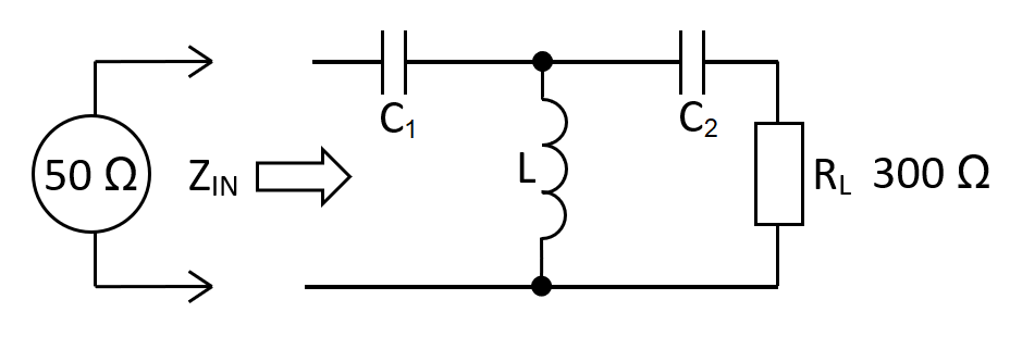
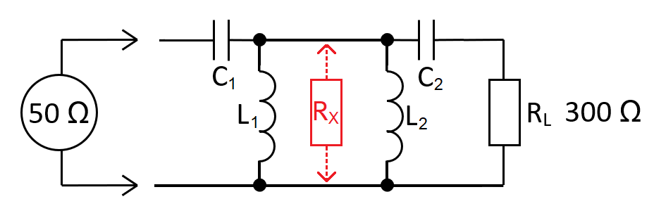
The high-pass T-network is equivalent to a pair of back-to-back high-pass L-Pad networks: -

$\hspace{18.9cm}$

High-pass T-network

Equivalent circuit

$C_1 = \dfrac{1}{\omega\cdot R_{IN}}\sqrt{\dfrac{1}{\frac{\color{red}{R_X}}{R_{IN}}-1}}\hspace{1cm} L_1 = C_1\cdot R_{IN}\cdot \color{red}{R_X} $

$C_2 = \dfrac{1}{\omega\cdot R_{L}}\sqrt{\dfrac{1}{\frac{\color{red}{R_X}}{R_L}-1}}\hspace{1.7cm} L_2 = C_2\cdot R_{L}\cdot\color{red}{R_X} $

The equivalent circuit

R_X represents $R_L$ for the left-stage and $R_{IN}$ for the right stage. You solve the left and right stages independently then combine L₁ and L₂ into inductor L_T. R_X is called the transfer impedance $Z_T$.

The calculator below requires R_IN to be less than R_X. This makes L₁ and C₁ an impedance multiplier with L₂ and C₂ as an impedance reducer. With the T calculator's default values, 50 Ω is converted to a $Z_T$ of 1000 Ω and then $Z_T$ is reduced to 300 Ω.

R_IN:		Ω
R_X:		Ω
R_L:		Ω
F_IN:		MHz
L₁:		µH
L₂:		µH
L_T:		µH
C₁:		pF
C₂:		pF
A_V at F_IN: Voltage gain from $Z_{IN}$ to $R_L$		V/V

The relevance of Q-factor

As previously proven for the basic L-Pad network, these relations are all true: - $$Q \hspace{0.5cm} = \hspace{0.5cm}A_V\hspace{0.5cm} = \hspace{0.5cm}\sqrt{\dfrac{R_L}{R_{IN}}}\hspace{0.5cm} = \hspace{0.5cm}R_L\sqrt{\dfrac{C}{L}}\hspace{0.5cm}=\hspace{0.5cm}\omega_n R_L C$$

This means that Q is not an input variable; it is wholly defined by $R_{IN}$ and $R_L$. However, because the T-network has a transfer impedance, Q-factor has two identities. For this reason, Q is discarded as an input variable in favour of R_X. $A_V$ is still calculated based on a lossless power transfer: - $$A_V=\sqrt{\dfrac{R_L}{R_{IN}}}$$

Benefits of the T-network

The 1st benefit is that you can manipulate the pass-bandwidth at the operating frequency. The image below shows the bode-plot response for several values of R_X. The upper graph is gain and the lower graphs are $\angle{Z_{IN}}$ and $|Z_{IN}|$: -

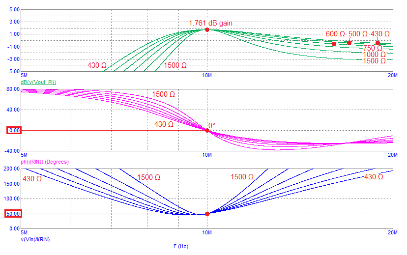
At 10 MHz, the gains converge at 1.761 dB. In real numbers that's 1.2247 and, when taking into account the 2:1 loss of connecting a 50 Ω source to a network with $Z_{IN}$ = 50 Ω, the voltage magnification is the same as the high-pass L-Pad network (2.44949): -

The 2nd benefit; The input impedance phase angle can be tailored to be more closely resistive than the L-Pad in the operating region around the centre frequency.

The 3rd benefit is that the input impedance and output impedance can be equal. This may not seem much of a benefit for an impedance transformer but, if you consider that several T-networks can be cascaded to produce a significant filtering effect, you have a tool that is very useful.

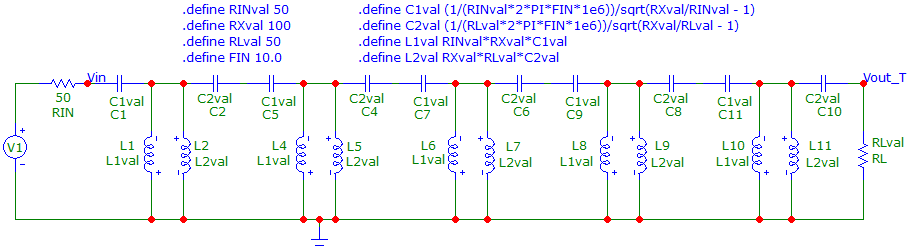
The high-pass T-network in cascade

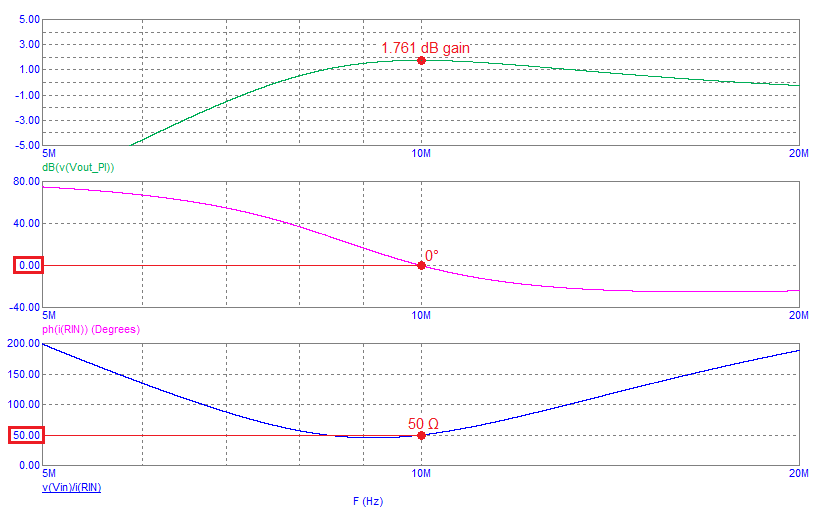
Below is a 50 Ω to 50 Ω, 5-stage cascaded T-network simulated in Micro-cap 12 (R_X = 100 Ω): -

The frequency response, impedance phase angle and impedance magnitude are below: -

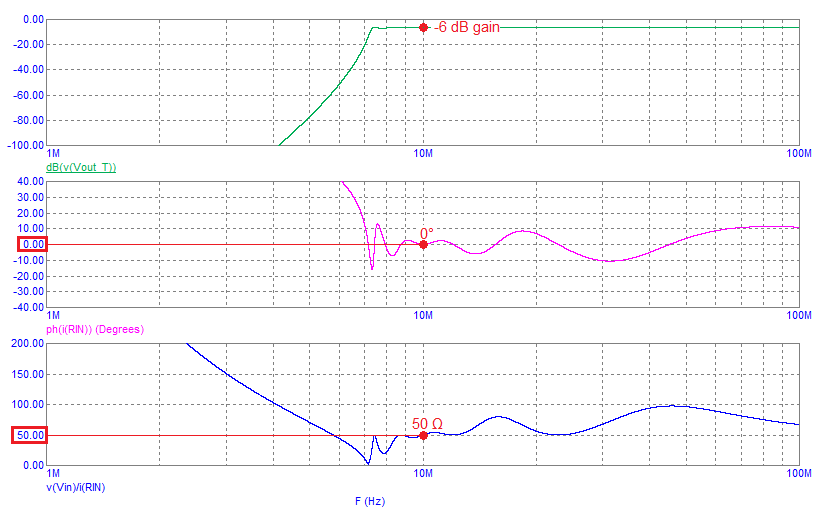
The main feature is the very sharp attenuation below about 7.5 MHz. $Z_{IN}$ is fairly flat from about 8.5 MHz to 13 MHz with its corresponding phase angle remaining close to 0° (resistive).

When cascading T stages, the value calculations are repeated and trivial.